
The dataset comes from the National Center for Education Statistics. In this article, I will demonstrate some data cleaning and dataframe manipulation techniques. Hope this helps!
For everything you may need, visit:
Source Data
nces-ed-attainment.csv
National Center for Education.py
The original dataset is titled: Percentage of persons 25 to 29 years old with selected levels of educational attainment, by race/ethnicity and sex: Selected years, 1920 through 2018. The cleaned version has columns for Year, Sex, Educational Attainment, and race/ethnicity categories considered in the dataset. Note that not all columns will have data starting at 1920.
Exploring the data
# packages needed
import pandas as pd
import pandas as pd
import numpy as np
import seaborn as sns
import matplotlib.pyplot as plt

df = pd.read_csv('nces-ed-attainment.csv')
df.head()
| Year | Sex | Min degree | Total | White | Black | Hispanic | Asian | Pacific Islander | American Indian/Alaska Native | Two or more races | |
|---|---|---|---|---|---|---|---|---|---|---|---|
| 0 | 1920 | A | high school | --- | 22.0 | 6.3 | --- | --- | --- | --- | --- | 1 | 1940 | A | high school | 38.1 | 41.2 | 12.3 | --- | --- | --- | --- | --- |
| 2 | 1950 | A | high school | 52.8 | 56.3 | 23.6 | --- | --- | --- | --- | --- |
| 3 | 1960 | A | high school | 60.7 | 63.7 | 38.6 | --- | --- | --- | --- | --- |
| 4 | 1970 | A | high school | 75.4 | 77.8 | 58.4 | --- | --- | --- | --- | --- |
df = df.replace('---', np.nan)
df.info()
<class 'pandas.core.frame.DataFrame'>
RangeIndex: 214 entries, 0 to 213
Data columns (total 11 columns):
 #   Column                         Non-Null Count  Dtype
---  ------                         --------------  -----
 0   Year                           214 non-null    int64
 1   Sex                            214 non-null    object
 2   Min degree                     214 non-null    object
 3   Total                          214 non-null    object
 4   White                          214 non-null    float64
 5   Black                          214 non-null    float64
 6   Hispanic                       214 non-null    object
 7   Asian                          214 non-null    object
 8   Pacific Islander               214 non-null    object
 9   American Indian/Alaska Native  214 non-null    object
 10  Two or more races              214 non-null    object
dtypes: float64(2), int64(1), object(8)
memory usage: 18.5+ KB
Several columns have wrong type.
race = [
    "Total",
    "Hispanic",
    "Asian",
    "Pacific Islander",
    "American Indian/Alaska Native",
    "Two or more races",
]
df[race] = df[race].apply(pd.to_numeric)
df.info()
<class 'pandas.core.frame.DataFrame'>
RangeIndex: 214 entries, 0 to 213
Data columns (total 11 columns):
 #   Column                         Non-Null Count  Dtype
---  ------                         --------------  -----
 0   Year                           214 non-null    int64
 1   Sex                            214 non-null    object
 2   Min degree                     214 non-null    object
 3   Total                          212 non-null    float64
 4   White                          214 non-null    float64
 5   Black                          214 non-null    float64
 6   Hispanic                       204 non-null    float64
 7   Asian                          168 non-null    float64
 8   Pacific Islander               93 non-null     float64
 9   American Indian/Alaska Native  131 non-null    float64
 10  Two or more races              157 non-null    float64
dtypes: float64(8), int64(1), object(2)
memory usage: 18.5+ KB
Have a look at some indicators of each column.
df.describe(include="all").T
| count | unique | top | freq | mean | std | min | 25% | 50% | 75% | max | |
|---|---|---|---|---|---|---|---|---|---|---|---|
| Year | 214.0 | NaN | NaN | NaN | 2005.48 | 15.6 | 1920.0 | 2005.0 | 2010.0 | 2014.0 | 2018.0 |
| Sex | 214 | 3 | A | 78 | NaN | NaN | NaN | NaN | NaN | NaN | NaN |
| Min degree | 214 | 4 | high school | 59 | NaN | NaN | NaN | NaN | NaN | NaN | NaN |
| Total | 212.0 | NaN | NaN | NaN | 42.77 | 30.15 | 4.1 | 22.12 | 36.1 | 84.4 | 94.0 |
| White | 214.0 | NaN | NaN | NaN | 47.21 | 31.32 | 4.5 | 22.3 | 42.65 | 85.9 | 96.4 |
| Black | 214.0 | NaN | NaN | NaN | 35.19 | 32.36 | 1.1 | 10.12 | 23.2 | 70.62 | 93.5 |
| Hispanic | 204.0 | NaN | NaN | NaN | 27.68 | 26.85 | 0.6 | 7.6 | 16.6 | 57.02 | 87.2 |
| Asian | 168.0 | NaN | NaN | NaN | 62.02 | 27.03 | 15.0 | 46.55 | 66.0 | 81.05 | 98.5 |
| Pacific Islander | 93.0 | NaN | NaN | NaN | 50.79 | 33.24 | 10.0 | 24.0 | 34.0 | 90.7 | 100.0 |
| American Indian/Alaska Native | 131.0 | NaN | NaN | NaN | 42.67 | 32.1 | 2.1 | 16.55 | 24.4 | 83.05 | 95.1 |
| Two or more races | 157.0 | NaN | NaN | NaN | 44.46 | 31.58 | 2.9 | 25.7 | 34.7 | 87.9 | 98.2 |
Visulization
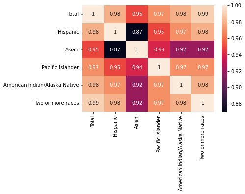
Correlation Matrix Heatmap
cormat = df[race].corr().round(2)
sns.heatmap(cormat, annot=True)
Enrollment Date Distribution
f, axes = plt.subplots(4, 2, sharey=False, figsize=(15, 12))
for ind, val in enumerate(race):
    sns.histplot(
        data=df,
        x=val,
        hue="Min degree",
        label="100% Equities",
        kde=True,
        stat="density",
        linewidth=0,
        ax=axes[ind // 2, ind % 2],
        bins=200,
    ).set(title=val)
f.tight_layout(pad=3.0)
plt.show()
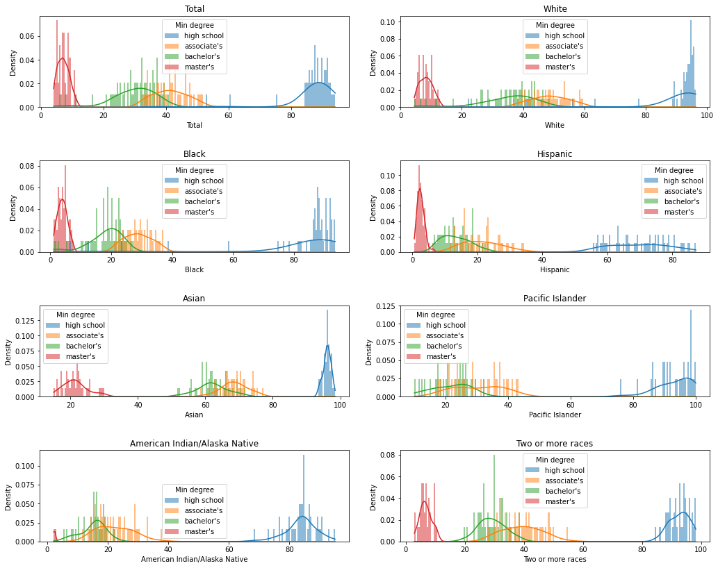
For Black, Hispanic, Pacific Islander people and people with two or more races, the enrollment rate is low for most of the past time. For Asian and White people, the overall enrollment rate is high for most of the past time.
f, axes = plt.subplots(4, 2, sharey=False, figsize=(14, 14))
for ind, val in enumerate(race):
    sns.lineplot(
        data=df, x="Year", y=val, hue="Min degree", ci=None, ax=axes[ind // 2, ind % 2]
    )
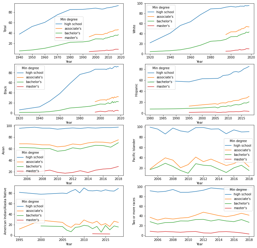
The Black and White people has low enrollment rate at the 1920s to 1970s, but the enrollments increased dramatically. For Black, White and Hispanic people, the enrollment rates for the four degrees has been increasing overtime. The enrollment rates of the four degrees keeps quite static since 2006 for Asian, Pacific Islander, American Indian/Alaska Native and people with two or more races.
Questions
Q1
What are the percent of different degrees completed for a given year range and sex? Parameter arguments are as follows: two year arguments, and a value for sex (’A’, ’F’, or ’M’). Function should return all rows of the data which match the given sex, and have data between the given years (inclusive for the start, exclusive for the end). If no data is found for the parameters, return Python keyword None.
def completion_bet_years(dataframe, year1, year2, sex):
    """ Return percent of different degrees completed between year1 and year2 for Sex==sex.

    Args:
    dataframe (DataFrame): A dataframe containing the needed data
    year1     (int)      : Year number: the  earlier one
    year2     (int)      : Year number: the  later one
    sex       (str)      : Gender

    Returns:
    DataFrame: The percent of degrees completed between year1 and year2 for Sex==sex.
    """
    result = dataframe.loc[
        (dataframe["Sex"] == sex)
        & (dataframe["Year"] >= year1)
        & (dataframe["Year"] < year2)
    ]
    if result.shape[0] == 0:
        return None
    else:
        return result

print(completion_bet_years(df, 1920, 1941, "A"))
    Year Sex   Min degree  Total  White  Black  Hispanic  Asian  \
0   1920   A  high school    NaN   22.0    6.3       NaN    NaN
1   1940   A  high school   38.1   41.2   12.3       NaN    NaN
39  1920   A   bachelor's    NaN    4.5    1.2       NaN    NaN
40  1940   A   bachelor's    5.9    6.4    1.6       NaN    NaN

    Pacific Islander  American Indian/Alaska Native  Two or more races
0                NaN                            NaN                NaN
1                NaN                            NaN                NaN
39               NaN                            NaN                NaN
40               NaN                            NaN                NaN
Q2
What were the percentages for women vs men having earned a Bachelor’s Degree in a given year? Parameter list argument is the year in question and return the percentages as a tuple: (% for men, % for women)
def compare_bachelors_in_year(dataframe, year):
    """ Return the percentages for women vs men having earned a Bachelor’s Degree in Year==year

    Args:
    df   (Dataframe): A dataframe containing the needed data
    year (int)      : The year in which you want to know the info

    Returns:
    tuple: A tuple returns the percentage of Bachelor’s Degree male and femal in Year==year.
    """
    women = dataframe[
        (dataframe["Sex"] == "F")
        & (dataframe["Min degree"] == "bachelor's")
        & (dataframe["Year"] == year)
    ].iloc[0]["Total"]
    men = dataframe[
        (dataframe["Sex"] == "M")
        & (dataframe["Min degree"] == "bachelor's")
        & (dataframe["Year"] == year)
    ].iloc[0]["Total"]
    return (f"{men} % for men", f"{women} % for women")

compare_bachelors_in_year(df, 2010)
('27.8 % for men', '35.7 % for women')
Q3
What were the two most commonly awarded levels of educational attainment awarded between 2000-2010 (inclusive)? Use the mean percent over the years to compare the education levels. Return a list as follows: [#1 level, mean % of #1 level, #2 level, mean % of #2 level].
def top_2_2000s(dataframe):
    """Return the two most common educational attainment between 2000-2010.

    Args:
    DataFrame (DataFrame): A dataframe containing the needed data

    Returns:
    list: A list returns the two most common educational attainment between 2000-2010.
    """
    df_2000s = dataframe.loc[
        (dataframe["Year"] >= 2000)
        & (dataframe["Year"] <= 2010)
        & (dataframe["Sex"] == "A")
    ][["Total", "Min degree"]]
    mean_percent_edu = (
        df_2000s.groupby("Min degree").mean().sort_values(by="Total", ascending=False)
    )
    level1 = mean_percent_edu.iloc[0]["Total"].round(2)
    level2 = mean_percent_edu.iloc[1]["Total"].round(2)
    edu1 = mean_percent_edu.index[0]
    edu2 = mean_percent_edu.index[1]
    return [f"#1 level, {level1} % of {edu1}", f"#2 level, {level2} % of {edu2}"]

top_2_2000s(df)
['#1 level, 87.557 % of high school', "#2 level, 38.757 % of associate's"]