import matplotlib.pyplot as plt
import seaborn as sns

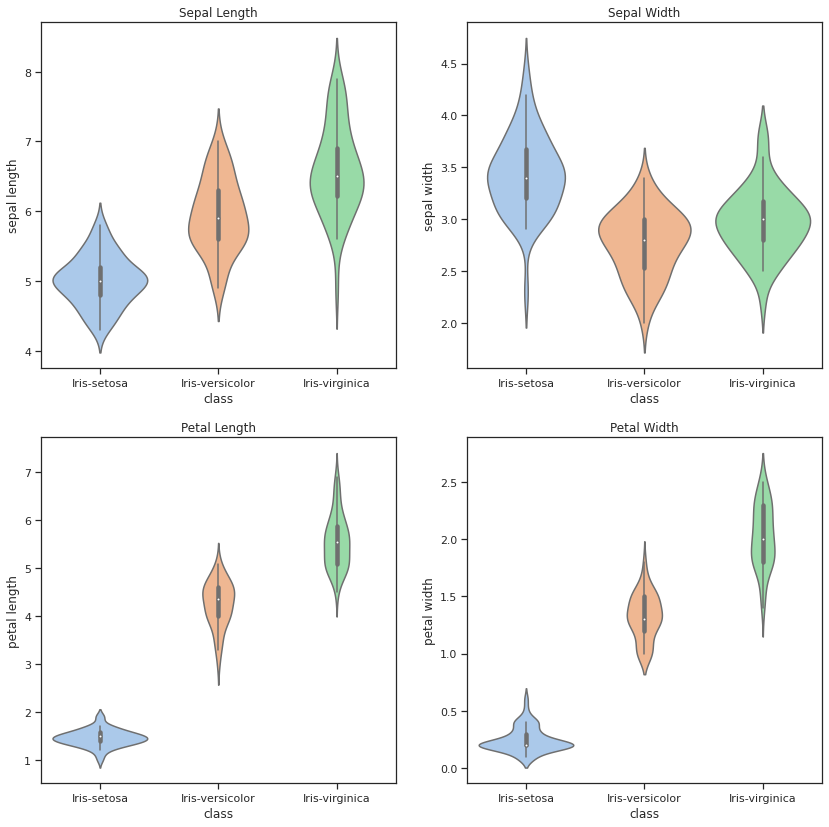
features = ["sepal length", "sepal width", "petal length", "petal width"]
sns.set(style="ticks", palette="pastel")
f, axes = plt.subplots(2, 2, sharey=False, figsize=(14, 14))
for ind, val in enumerate(features):
    sns.violinplot(x="class", y=val, data=df, ax=axes[ind // 2, ind % 2]).set(
        title = "Sepal Length"
    )

plt.show()

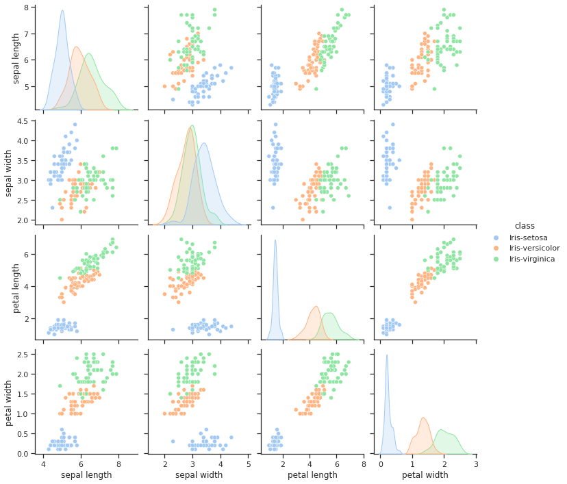
sns.pairplot(df, hue="class")

Train and evaluate three models using cross-validation

K-Nearest Neighbors Classifier

from sklearn.preprocessing import StandardScaler
from sklearn.neighbors import KNeighborsClassifier
from sklearn.model_selection import ShuffleSplit
from sklearn.preprocessing import StandardScaler
from sklearn.pipeline import Pipeline
from sklearn.model_selection import GridSearchCV

NUM         = 200
X           = df.drop(["class"], axis=1)
y           = df["class"]
shuffle     = ShuffleSplit(n_splits=NUM, test_size=0.25, random_state=10)
results     = []
klist       = np.arange(1, 21, 1)
FullModel   = Pipeline([("scaler", StandardScaler()), ("knn", KNeighborsClassifier())])
param_grid  = {"knn__n_neighbors": klist}
grid_search = GridSearchCV(
    FullModel,
    param_grid,
    scoring            = "accuracy",
    cv                 = shuffle,
    return_train_score = True,
    n_jobs             = -1,
)
grid_search.fit(X, y)
results = pd.DataFrame(grid_search.cv_results_)

print(
    results[
        [
            "rank_test_score",
            "mean_train_score",
            "mean_test_score",
            "param_knn__n_neighbors",
        ]
    ]
)

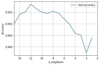
# Plot Accuracy vs K
fig, ax = plt.subplots()
ax.plot(
    results["param_knn__n_neighbors"], results["mean_test_score"], label="test accuracy"
)
ax.set_xlim(15, 0)  # reverse x; from simple model to complex model
# (complex model tries hard to sort of figure out all sorts of details in the data)
ax.set_ylabel("Accuracy")
ax.set_xlabel("n_neighbors")
ax.grid()
ax.legend()

Naive Bayes Classifier

from sklearn.naive_bayes import MultinomialNB
from sklearn.preprocessing import MinMaxScaler
features = ["sepal length", "sepal width", "petal length", "petal width"]

df1 = df.copy()
for column in features:
    df1[column] = [round(i - np.min(df1[column])) for i in df1[column]]
    df1[column] = df1[column].astype("category")
    X = pd.get_dummies(df1[features])

# Calculate mean test accuracy
alphas      = [0.01, 0.1, 1.0, 5.0, 10.0, 15.0, 20.0, 35.0, 50.0]
FullModel   = Pipeline([("scaler", MinMaxScaler()), ("mnb", MultinomialNB())])
param_grid  = {"mnb__alpha": alphas}
grid_search = GridSearchCV(
    FullModel,
    param_grid,
    scoring            = "accuracy",
    cv                 = shuffle,
    return_train_score = True,
    n_jobs             = -1,
)
grid_search.fit(X, y)
results = pd.DataFrame(grid_search.cv_results_)
print(
    results[
        ["rank_test_score", "mean_train_score", "mean_test_score", "param_mnb__alpha"]
    ]
)

Logistic Regression

from sklearn.linear_model import LogisticRegression

df2 = df.copy()
X   = df2.iloc[:, 0:4].values
y   = df2.iloc[:, 4].values

# Calculate mean test accuracy
Clist     = [0.01, 0.1, 1.0, 5.0, 10.0, 20.0, 50.0, 100.0, 150.0, 200.0]
FullModel = Pipeline(
    [
        ("scaler", StandardScaler()),
        ("lr", LogisticRegression(penalty="l2", solver="lbfgs", multi_class="auto")),
    ]
)
param_grid  = {"lr__C": Clist}
grid_search = GridSearchCV(
    FullModel,
    param_grid,
    scoring            = "accuracy",
    cv                 = shuffle,
    return_train_score = True,
    n_jobs             = -1,
)
grid_search.fit(X, y)
results = pd.DataFrame(grid_search.cv_results_)
print(
    results[["rank_test_score", "mean_train_score", "mean_test_score", "param_lr__C"]]
)

Conclusion

For the current running, Logistic Regression has the highest test accuracy followed by KNN Classifier. Naive Bayes Classifier has the lowest test accuracy.