
This is a thorough analysis of diabetes dataset from Kaggle. In this article, I will demonstrate how to do an end-to-end machine learning project using diverse classification models including K-Nearest Neighbors, Logistic Regression, Support Vector Machine, Decision Tree and Random Forest.
For everything you may need, visit:
Source Data
Hope this helps!
I cannot emphasize the importance of data preprocessing. It is the process of transforming raw data into more reasonable, useful and efficient format. It's a must and one of the most important step in a machine learing project. Without it our models will probably crash and won't be able to generate good results.
There are several steps in data preprocessing: data cleaning, data reduction and data transformation. In the following paragraphs, I'll show you how to perform the steps one by one.
Data Cleaning
First, I load the data from the .csv file and print the first ten rows so that I can have a basic understanding of how the data looks like.
# packages needed
import numpy as np
import pandas as pd

# load data
data = pd.read_csv('diabetes.csv')
data.head(10)
| Pregnancies | Glucose | BloodPressure | SkinThickness | Insulin | BMI | DiabetesPedigreeFunction | Age | Outcome | |
|---|---|---|---|---|---|---|---|---|---|
| 0 | 6 | 148 | 72 | 35 | 0 | 33.6 | 0.627 | 50 | 1 |
| 1 | 1 | 85 | 66 | 29 | 0 | 26.6 | 0.351 | 31 | 0 |
| 2 | 8 | 183 | 64 | 0 | 0 | 23.3 | 0.672 | 32 | 1 |
| 3 | 1 | 89 | 66 | 23 | 94 | 28.1 | 0.167 | 21 | 0 |
| 4 | 0 | 137 | 40 | 35 | 168 | 43.1 | 2.288 | 33 | 1 |
| 5 | 5 | 116 | 74 | 0 | 0 | 25.6 | 0.201 | 30 | 0 |
| 6 | 3 | 78 | 50 | 32 | 88 | 31.0 | 0.248 | 26 | 1 |
| 7 | 10 | 115 | 0 | 0 | 0 | 35.3 | 0.134 | 29 | 0 |
| 8 | 2 | 197 | 70 | 45 | 543 | 30.5 | 0.158 | 53 | 1 |
| 9 | 8 | 125 | 96 | 0 | 0 | 0.0 | 0.232 | 54 | 1 |
The meaning of each column is stated as below:
- Pregnancies: Number of times pregnant
- Glucose: Plasma glucose concentration a 2 hours in an oral glucose tolerance test
- BloodPressure: Diastolic blood pressure (mm Hg)
- SkinThickness: Triceps skin fold thickness (mm)
- Insulin: 2-Hour serum insulin (mu U/ml)
- BMI: Body mass index (weight in kg/(height in m)^2)
- DiabetesPedigreeFunction: Diabetes pedigree function
- Age: Age (years)
- Outcome: Class variable (0 or 1)
Next, we need to examin whether there are null values in the dataset.
data.isnull().sum()
Pregnancies                 0
Glucose                     0
BloodPressure               0
SkinThickness               0
Insulin                     0
BMI                         0
DiabetesPedigreeFunction    0
Age                         0
Outcome                     0
dtype: int64
It seems there is no null values. Shall we pop the champagne now? If we further examine the data, we will find that the situation is not as good as we thought.
data.describe().round(2).T
| count | mean | std | min | 25% | 50% | 75% | max | |
|---|---|---|---|---|---|---|---|---|
| Pregnancies | 768.0 | 3.85 | 3.37 | 0.00 | 1.00 | 3.00 | 6.00 | 17.00 |
| Glucose | 768.0 | 120.89 | 31.97 | 0.00 | 99.00 | 117.00 | 140.25 | 199.00 |
| BloodPressure | 768.0 | 69.11 | 19.36 | 0.00 | 62.00 | 72.00 | 80.00 | 122.00 |
| SkinThickness | 768.0 | 20.54 | 15.95 | 0.00 | 0.00 | 23.00 | 32.00 | 99.00 |
| Insulin | 768.0 | 79.80 | 115.24 | 0.00 | 0.00 | 30.50 | 127.25 | 846.00 |
| BMI | 768.0 | 31.99 | 7.88 | 0.00 | 27.30 | 32.00 | 36.60 | 67.10 |
| DiabetesPedigreeFunction | 768.0 | 0.47 | 0.33 | 0.08 | 0.24 | 0.37 | 0.63 | 2.42 |
| Age | 768.0 | 33.24 | 11.76 | 21.00 | 24.00 | 29.00 | 41.00 | 81.00 |
| Outcome | 768.0 | 0.35 | 0.48 | 0.00 | 0.00 | 0.00 | 1.00 | 1.00 |
for col in list(data.columns):
    zero = len(data[data[col] == 0])
    print('0s in %s: %d' % (col, zero))
0s in Pregnancies: 111
0s in Glucose: 5
0s in BloodPressure: 35
0s in SkinThickness: 227
0s in Insulin: 374
0s in BMI: 11
0s in DiabetesPedigreeFunction: 0
0s in Age: 0
0s in Outcome: 500
There are nearly 400 null values in Insulin column, so it's not realistic to drop all the null values. Normally under such circumstance, we replace them with indicators such as mean, median, or mode, etc. Here I choose median.
# replace 0s in target columns with null value
data.iloc[:, 1:6] = data.iloc[:, 1:6].replace({0:np.NaN})
# fill null values with medians
data = data.fillna(data.median())
data.describe().round(2).T
| count | mean | std | min | 25% | 50% | 75% | max | |
|---|---|---|---|---|---|---|---|---|
| Pregnancies | 768.0 | 3.85 | 3.37 | 0.00 | 1.00 | 3.00 | 6.00 | 17.00 |
| Glucose | 768.0 | 121.66 | 30.44 | 44.00 | 99.75 | 117.00 | 140.25 | 199.00 |
| BloodPressure | 768.0 | 72.39 | 12.10 | 24.00 | 64.00 | 72.00 | 80.00 | 122.00 |
| SkinThickness | 768.0 | 29.11 | 8.79 | 7.00 | 25.00 | 29.00 | 32.00 | 99.00 |
| Insulin | 768.0 | 140.67 | 86.38 | 14.00 | 121.50 | 125.00 | 127.25 | 846.00 |
| BMI | 768.0 | 32.46 | 6.88 | 18.20 | 27.50 | 32.30 | 36.60 | 67.10 |
| DiabetesPedigreeFunction | 768.0 | 0.47 | 0.33 | 0.08 | 0.24 | 0.37 | 0.63 | 2.42 |
| Age | 768.0 | 33.24 | 11.76 | 21.00 | 24.00 | 29.00 | 41.00 | 81.00 |
| Outcome | 768.0 | 0.35 | 0.48 | 0.00 | 0.00 | 0.00 | 1.00 | 1.00 |
Pairplot & Correlation Matrix -- Imbalanced Dataset
Now we can visualize the dataset and see if we can find something else.
import seaborn as sns
import matplotlib.pyplot as plt
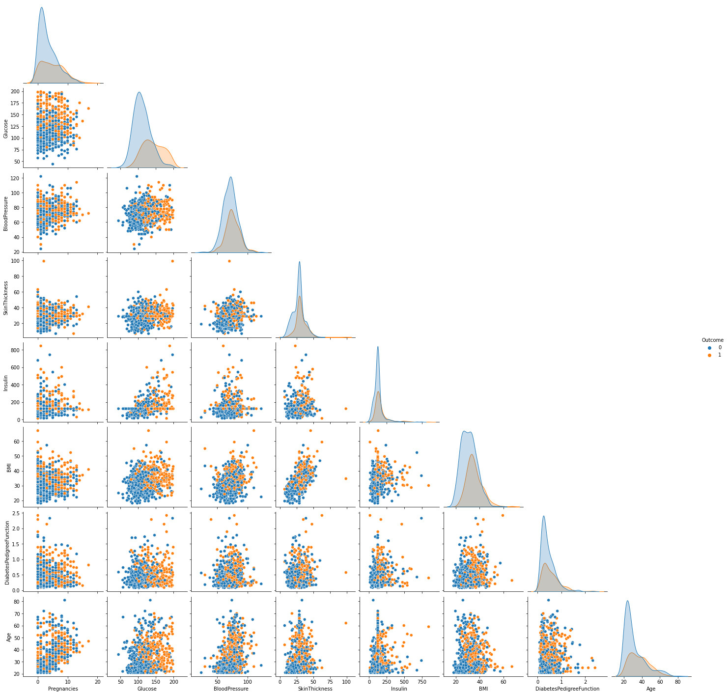
sns.pairplot(data, hue="Outcome", corner=True)
corr_mat = data.corr().round(2)
plt.figure(figsize = (15,10))
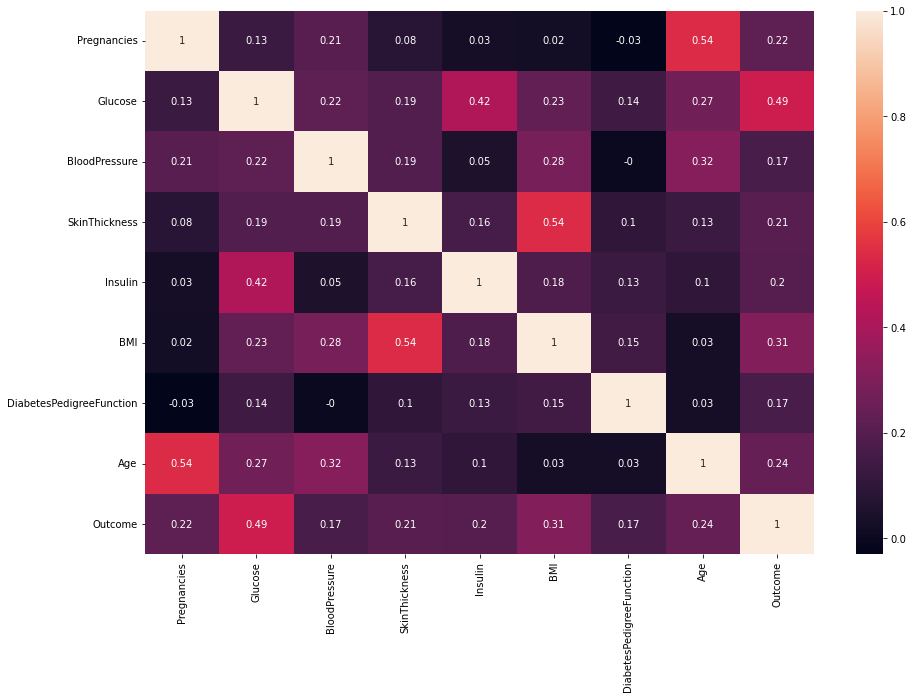
sns.heatmap(corr_mat, annot=True)
From the pairplot above, we discover this is an imbalanced dataset. There are 500 observations whose outcome is 0 and only 268 is 1. If we train our model with such data, the results may be misleading. There are several methods to deal with imbalanced data:
- Collect more data
- Under-Sampling
- Over-Sampling
- Use confusion matrix or other ways to evaluate the peformance
As the number of observations is only 768, it's unrealistic to under-sampling. Here I wil illustrate how to do oversampling using SMOTE().
Oversampling with SMOTE()
We can use SMOTE() to over-sampling observations so that the number of outcome in each class will be the same. After doing that, we describe the data again.
from imblearn.over_sampling import SMOTE
# get X, y
X          = data.iloc[:, 0:8]
y          = data.iloc[:, -1]
# perform SMOTE()
oversample = SMOTE()
X, y       = oversample.fit_resample(X, y)
# join X, y
y          = pd.DataFrame(y)
data       = pd.concat([X, y], axis=1)
print(data.shape)
data.describe().round(2).T
| count | mean | std | min | 25% | 50% | 75% | max | |
|---|---|---|---|---|---|---|---|---|
| Pregnancies | 1000.0 | 3.99 | 3.33 | 0.00 | 1.00 | 3.00 | 6.00 | 17.00 |
| Glucose | 1000.0 | 126.40 | 31.39 | 44.00 | 102.82 | 122.00 | 148.00 | 199.00 |
| BloodPressure | 1000.0 | 72.97 | 11.71 | 24.00 | 65.75 | 72.00 | 80.00 | 122.00 |
| SkinThickness | 1000.0 | 29.64 | 8.22 | 7.00 | 27.00 | 29.00 | 33.00 | 99.00 |
| Insulin | 1000.0 | 146.58 | 90.69 | 14.00 | 125.00 | 125.00 | 136.25 | 846.00 |
| BMI | 1000.0 | 33.01 | 6.68 | 18.20 | 28.40 | 32.66 | 36.80 | 67.10 |
| DiabetesPedigreeFunction | 1000.0 | 0.49 | 0.32 | 0.08 | 0.26 | 0.40 | 0.65 | 2.42 |
| Age | 1000.0 | 33.88 | 11.34 | 21.00 | 25.00 | 31.00 | 41.00 | 81.00 |
| Outcome | 1000.0 | 0.50 | 0.50 | 0.00 | 0.00 | 0.50 | 1.00 | 1.00 |
Pairplot & Correlation Matrix -- Balanced Dataset
Once again visualize the dataset to see the changes in the distribution of data.
sns.pairplot(data, hue="Outcome", corner=True)

For now, we transform the original imbalanced dataset into a balanced dataset with the number of each outcome class being 500. there is not much difference in distribution between diabetics and nondiabetics. Glucose should have the highest correlation with Outcome among all the features. We can testify it using a correlation matrix heatmap.
corr_mat = data.corr().round(2)
plt.figure(figsize = (15,10))
sns.heatmap(corr_mat, annot=True)
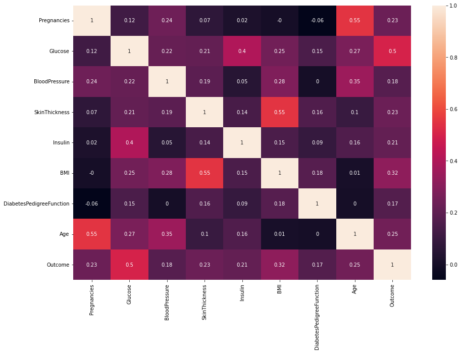
The features with higher correlation with Outcome are more important and more inspirable to our model process.
Data Transformation
If the range of two features differ a lot, for example, one is from 0 to 1 and the other is from 0 to 10,000, apparantly models won't treat such two features equally. Normally, the feature with larger range would influence the result more. Nevertheless, this doesn't mean it's more important than the other one. That's why we need scale the features. Frequently used scaling techniques are:
- MinMaxScaler()
- StardardScaler()
- MaxAbsScaler()
- RobustScaler()
I usually choose MinMaxScaler() or StandardScaler() for most of datasets. You can also use others according to the charasteristic of the dataset at hand.
from sklearn.model_selection import train_test_split
from sklearn.preprocessing import StandardScaler

# get X, y
X  = data.drop(["Outcome"], axis=1)
y  = data["Outcome"]

X2 = X.copy
y2 = y.copy

# split X, y into traning set and validation set
X2_train, X2_trainValid, y2_train, y2_trainValid = train_test_split(X2, y2, test_size=0.5)
# perform feature scaling
scaler   = StandardScaler()

X2_train = scaler.fit_transform(X2_train)
print("The training set:")
print(X2_train)

X2_trainValid = scaler.transform(X2_trainValid)
print("The validation set:")
print(X2_trainValid)
The training set:
[[ 0.91861577  1.16692299  1.18785055 ... -0.37252998 -1.00546758
   1.12702163]
 [-0.31857719  2.14006051 -0.37791467 ... -0.29655845 -0.59256699
  -0.00540078]
 [-1.2464719  -0.54138673  1.3123182  ... -0.07795059  0.92337497
   0.25592747]
 ...
 [ 0.60931753  0.71279215  0.66592881 ... -0.50927873 -0.96541006
   1.38834988]
 [ 0.91861577  0.69093641  0.49301433 ...  0.36541497  0.17583587
   1.4754593 ]
 [-1.2464719  -1.00641748 -0.20394076 ...  1.61792412 -0.44466231
  -1.1378232 ]]
The validation set:
[[-0.93717366 -1.13616915 -0.89983642 ... -0.85874777  0.2732917
  -0.87649495]
 [-0.62787543 -1.03885539 -0.7258625  ...  0.78223728  0.56293838
  -0.96360437]
 [ 0.30001929 -1.20104498 -0.55188859 ... -1.28418834 -0.46006904
  -0.35383845]
 ...
 [-0.62787543 -0.94154164 -0.37791467 ... -1.78560044  0.47974199
  -0.70227612]
 [ 0.30001929  0.61547839  0.83990272 ... -0.12942108 -0.1211208
   2.08522521]
 [ 0.60931753 -0.58472455  1.36182446 ...  0.59990561  0.72624981
  -0.26672903]]
Data Reduction
With clean data at hand, we can visulize the data, which may indicate some relations between the features or between features and targets. Knowing these is useful to data reduction, for example, if a feature is highly correlated with the target, then we had better retain it. Or if two features are highly correlated, it would be much easier for us if we drop out one of them. Here I use PCA (Principal componenet analysis) for a demonstration.
from sklearn.decomposition import PCA

pca      = PCA()

X2_train = pca.fit_transform(X2_train)
print("The training set:")
print(X2_train)

X2_trainValid = pca.transform(X2_trainValid)
print("The validation set:")
print(X2_trainValid)
The training set:
[[ 1.11094069  1.71567637  0.06106008 ... -0.41295852  0.00731795
  -0.44959938]
 [-0.35117318  0.31229466  1.6917659  ... -1.61109567 -0.49354468
   0.3728086 ]
 [ 0.16735037 -0.4001708  -0.38262459 ...  0.82802415  0.95458562
  -0.10766268]
 ...
 [ 0.66464415  1.65681528  0.09661504 ... -0.34339558  0.49824185
  -0.21578121]
 [ 1.89124805  0.9469956   0.91665363 ...  0.40528492  0.16728102
   0.47349385]
 [-0.77480095 -1.71331367 -1.18697513 ...  0.26478707 -0.22960668
   1.25339887]]
The validation set:
[[-2.92512666 -0.09229361  0.31554059 ... -0.10102492 -0.22291171
   0.68989167]
 [-0.55971697 -1.49656753 -0.53947916 ...  0.41658342 -0.12598596
   0.48539238]
 [-2.27295931  1.03707233 -0.42829519 ... -0.03041183 -0.23491582
  -0.2007138 ]
 ...
 [-2.79570134  0.52778715  0.64923584 ...  0.15441194 -0.14783737
  -0.13731851]
 [ 1.54801396  1.38771828  1.28965127 ...  0.67922686  0.85859194
   0.66502772]
 [ 0.65313216  0.2231839  -0.87818227 ...  0.76275166 -0.74002896
   0.09427758]]