In the previous article, I analyze the bike sharing dataset from a daily level. In this article, I will do a similar procedure from a houly level.
Source data: hour.csv
Source python file: Bike Sharing Dataset Analytics -- Hourly Data.py
Exploring the Data
import pandas as pd
hour = pd.read_csv("hour.csv")
hour.head()
|
instant |
dteday |
season |
yr |
mnth |
hr |
holiday |
weekday |
workingday |
weathersit |
temp |
atemp |
hum |
windspeed |
casual |
registered |
cnt |
| 0 |
1 |
2011-01-01 |
1 |
0 |
1 |
0 |
0 |
6 |
0 |
1 |
0.24 |
0.2879 |
0.81 |
0.0 |
3 |
13 |
16 |
| 1 |
2 |
2011-01-01 |
1 |
0 |
1 |
1 |
0 |
6 |
0 |
1 |
0.22 |
0.2727 |
0.80 |
0.0 |
8 |
32 |
40 |
| 2 |
3 |
2011-01-01 |
1 |
0 |
1 |
2 |
0 |
6 |
0 |
1 |
0.22 |
0.2727 |
0.80 |
0.0 |
5 |
27 |
32 |
| 3 |
4 |
2011-01-01 |
1 |
0 |
1 |
3 |
0 |
6 |
0 |
1 |
0.24 |
0.2879 |
0.75 |
0.0 |
3 |
10 |
13 |
| 4 |
5 |
2011-01-01 |
1 |
0 |
1 |
4 |
0 |
6 |
0 |
1 |
0.24 |
0.2879 |
0.75 |
0.0 |
0 |
1 |
1 |
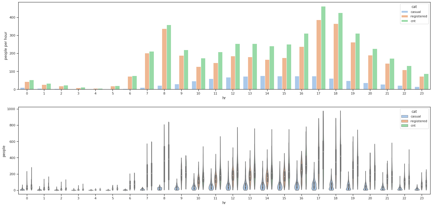
Visualization
import matplotlib.pyplot as plt
result = hour[["hr", "casual", "registered", "cnt"]].groupby(["hr"]).mean()
result = (
    result.stack()
    .reset_index()
    .set_index("hr")
    .rename(columns={"level_1": "cat", 0: "people per hour"})
)
f, axes = plt.subplots(2, sharey=False, figsize=(25, 12))
sns.barplot(x=result.index, y="people per hour", hue="cat", data=result, ax=axes[0])

result = hour[["casual", "registered", "cnt"]].set_index(hour["hr"])
result = (
    result.stack()
    .reset_index()
    .set_index("hr")
    .rename(columns={"level_1": "cat", 0: "people"})
)
sns.violinplot(x=result.index, y="people", hue="cat", data=result, cut=0, ax=axes[1])
Linear Regression
Split Data
from sklearn.model_selection import train_test_split
from sklearn.preprocessing import StandardScaler

cat       = ["season", "mnth", "hr", "holiday", "weekday", "workingday", "weathersit"]
hour[cat] = hour[cat].apply(lambda x: x.astype("category"))
dummies   = pd.get_dummies(hour[cat], drop_first=True)
print(dummies.shape)
conti_predictors = ["temp", "atemp", "hum", "windspeed"]
print(hour[conti_predictors].shape)
X = pd.concat([hour[conti_predictors], dummies], axis=1)
X.head()
y = hour.iloc[:, 14:]
y.head()

X_train, X_test, y_train, y_test = train_test_split(X, y, test_size=0.25)
sc = StandardScaler()
X_train[conti_predictors] = sc.fit_transform(X_train[conti_predictors])
X_test[conti_predictors] = sc.transform(X_test[conti_predictors])
(17379, 48)
(17379, 4)
|
temp |
atemp |
hum |
windspeed |
season_2 |
season_3 |
season_4 |
mnth_2 |
mnth_3 |
mnth_4 |
mnth_5 |
mnth_6 |
mnth_7 |
mnth_8 |
mnth_9 |
mnth_10 |
mnth_11 |
mnth_12 |
hr_1 |
hr_2 |
hr_3 |
hr_4 |
hr_5 |
hr_6 |
hr_7 |
hr_8 |
hr_9 |
hr_10 |
hr_11 |
hr_12 |
hr_13 |
hr_14 |
hr_15 |
hr_16 |
hr_17 |
hr_18 |
hr_19 |
hr_20 |
hr_21 |
hr_22 |
hr_23 |
holiday_1 |
weekday_1 |
weekday_2 |
weekday_3 |
weekday_4 |
weekday_5 |
weekday_6 |
workingday_1 |
weathersit_2 |
weathersit_3 |
weathersit_4 |
| 0 |
0.24 |
0.2879 |
0.81 |
0.0 |
0 |
0 |
0 |
0 |
0 |
0 |
0 |
0 |
0 |
0 |
0 |
0 |
0 |
0 |
0 |
0 |
0 |
0 |
0 |
0 |
0 |
0 |
0 |
0 |
0 |
0 |
0 |
0 |
0 |
0 |
0 |
0 |
0 |
0 |
0 |
0 |
0 |
0 |
0 |
0 |
0 |
0 |
0 |
1 |
0 |
0 |
0 |
0 |
| 1 |
0.22 |
0.2727 |
0.80 |
0.0 |
0 |
0 |
0 |
0 |
0 |
0 |
0 |
0 |
0 |
0 |
0 |
0 |
0 |
0 |
1 |
0 |
0 |
0 |
0 |
0 |
0 |
0 |
0 |
0 |
0 |
0 |
0 |
0 |
0 |
0 |
0 |
0 |
0 |
0 |
0 |
0 |
0 |
0 |
0 |
0 |
0 |
0 |
0 |
1 |
0 |
0 |
0 |
0 |
| 2 |
0.22 |
0.2727 |
0.80 |
0.0 |
0 |
0 |
0 |
0 |
0 |
0 |
0 |
0 |
0 |
0 |
0 |
0 |
0 |
0 |
0 |
1 |
0 |
0 |
0 |
0 |
0 |
0 |
0 |
0 |
0 |
0 |
0 |
0 |
0 |
0 |
0 |
0 |
0 |
0 |
0 |
0 |
0 |
0 |
0 |
0 |
0 |
0 |
0 |
1 |
0 |
0 |
0 |
0 |
| 3 |
0.24 |
0.2879 |
0.75 |
0.0 |
0 |
0 |
0 |
0 |
0 |
0 |
0 |
0 |
0 |
0 |
0 |
0 |
0 |
0 |
0 |
0 |
1 |
0 |
0 |
0 |
0 |
0 |
0 |
0 |
0 |
0 |
0 |
0 |
0 |
0 |
0 |
0 |
0 |
0 |
0 |
0 |
0 |
0 |
0 |
0 |
0 |
0 |
0 |
1 |
0 |
0 |
0 |
0 |
| 4 |
0.24 |
0.2879 |
0.75 |
0.0 |
0 |
0 |
0 |
0 |
0 |
0 |
0 |
0 |
0 |
0 |
0 |
0 |
0 |
0 |
0 |
0 |
0 |
1 |
0 |
0 |
0 |
0 |
0 |
0 |
0 |
0 |
0 |
0 |
0 |
0 |
0 |
0 |
0 |
0 |
0 |
0 |
0 |
0 |
0 |
0 |
0 |
0 |
0 |
1 |
0 |
0 |
0 |
0 |
|
casual |
registered |
cnt |
| 0 |
3 |
13 |
16 |
| 1 |
8 |
32 |
40 |
| 2 |
5 |
27 |
32 |
| 3 |
3 |
10 |
13 |
| 4 |
0 |
1 |
1 |
Train Model
from sklearn.linear_model import LinearRegression
from dmba import adjusted_r2_score

lr = LinearRegression()
lr.fit(X_train, y_train)

y_pred = lr.predict(X_test)
y_pred = pd.DataFrame(y_pred, columns=["casual", "registered", "cnt"]).astype(int)
print(y_pred)
print(adjusted_r2_score(y_test, y_pred, lr))
|
casual |
registered |
cnt |
| 0 |
37 |
249 |
286 |
| 1 |
42 |
344 |
386 |
| 2 |
48 |
259 |
307 |
| 3 |
19 |
360 |
380 |
| 4 |
-9 |
-88 |
-98 |
| ... |
... |
... |
... |
| 4340 |
6 |
205 |
211 |
| 4341 |
6 |
109 |
115 |
| 4342 |
32 |
226 |
259 |
| 4343 |
52 |
93 |
146 |
| 4344 |
-5 |
142 |
137 |
0.5979873068757086
Because number of people cannot be negative, we change some data so that the result make sense.
for i in range(y_pred.shape[0]):
    if y_pred["casual"].iloc[i] < 0:
        y_pred["casual"].iloc[i] = 0
    if y_pred["registered"].iloc[i] < 0:
        y_pred["registered"].iloc[i] = 0
        y_pred["cnt"].iloc[i] = y_pred["casual"].iloc[i] + y_pred["registered"].iloc[i]
print(y_pred)
print(adjusted_r2_score(y_test, y_pred, lr))
|
casual |
registered |
cnt |
| 0 |
37 |
249 |
286 |
| 1 |
42 |
344 |
386 |
| 2 |
48 |
259 |
307 |
| 3 |
19 |
360 |
380 |
| 4 |
0 |
0 |
0 |
| ... |
... |
... |
... |
| 4340 |
6 |
205 |
211 |
| 4341 |
6 |
109 |
115 |
| 4342 |
32 |
226 |
259 |
| 4343 |
52 |
93 |
146 |
| 4344 |
0 |
142 |
142 |
0.6153434162490663